


Financial Analytics & Automation / Power BI KPI Dashboard Creation Series
Introduction
In Vol. 2, we covered how to install Power BI Desktop and explored its main interface. You should now have a basic understanding of key areas such as the Ribbon, Report Canvas, and Data pane.
In this article, we will import data into Power BI to prepare the data foundation needed for our KPI calculations.
Sample Data Used in This Article
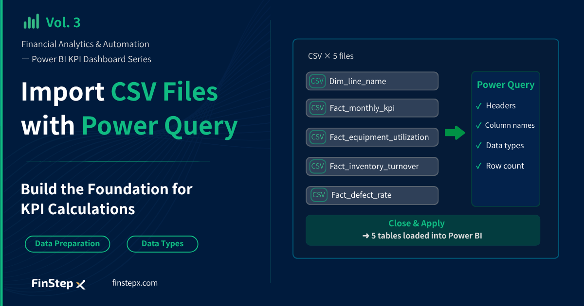
In real-world business environments, the data required for analysis is often spread across multiple files or database tables. To simulate this type of environment, we will use the following five CSV files. The structure has been kept simple so that it’s easy for you to follow in this series.
Download the sample data
| File Name | Contents | Columns |
|---|---|---|
Dim_line_name.csv | Production line master data | LineName |
Fact_monthly_kpi.csv | Revenue and cost data | Year/Month Line Name Net Sales COGS SG&A Target Operating Margin |
Fact_equipment_utilization.csv | Equipment utilization data | Year/Month Line Name Utilization Rate Target Utilization Rate |
Fact_inventory_turnover.csv | Inventory turnover data | Year/Month Line Name Product Category Beginning Inventory Purchases Ending Inventory COGS Target Inventory Turnover |
Fact_defect_rate.csv | Defect rate data | Year/Month Line Name Production Quantity Defect Quantity Target Defect Rate |
Step 1: Save the Power BI File
Before starting the data preparation process, save your Power BI file first.
In practice, it is a good habit to save your file at the beginning of your work and periodically press Ctrl + S to save the updates. This helps ensure that your work is preserved if something goes wrong during the process.
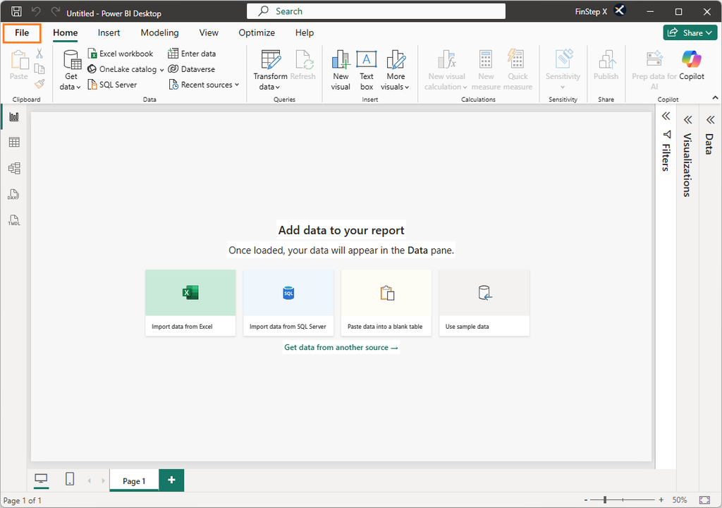
With the Blank report opened from Vol. 2, click File.
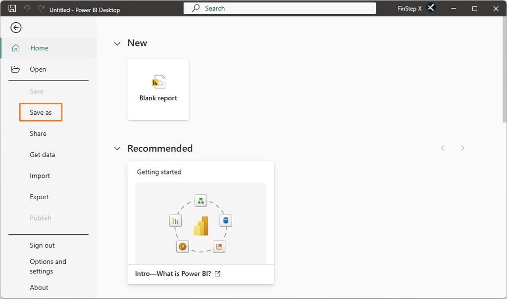
On the next screen, click Save As.
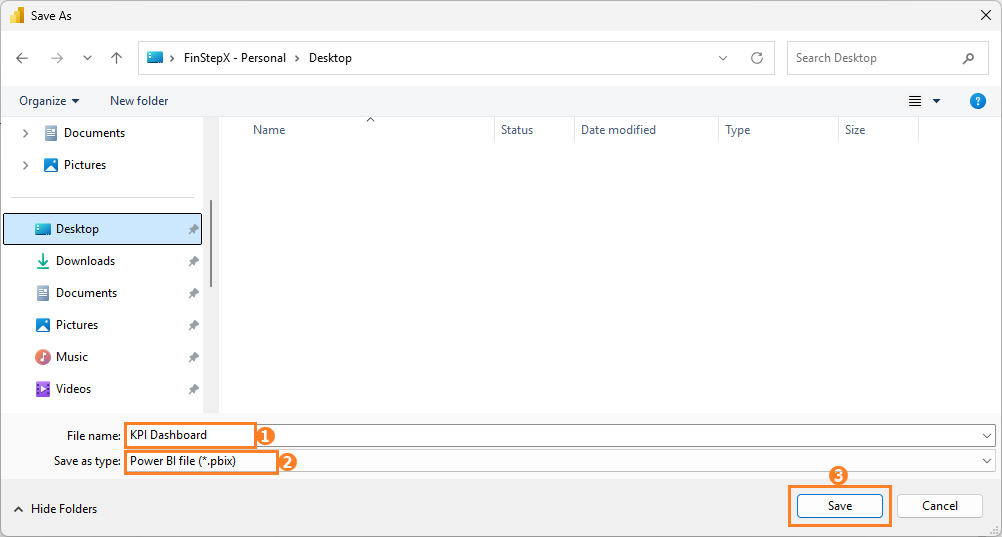
In the file save dialog, enter KPI Dashboard as the file name and make sure the file type is set to Power BI file (*.pbix). Click Save.
After saving the Power BI file, the file name and save time will be displayed at the top of the Power BI Desktop window.
Step 2: Import the First CSV File with Power Query
Let’s start by importing the first sample file.
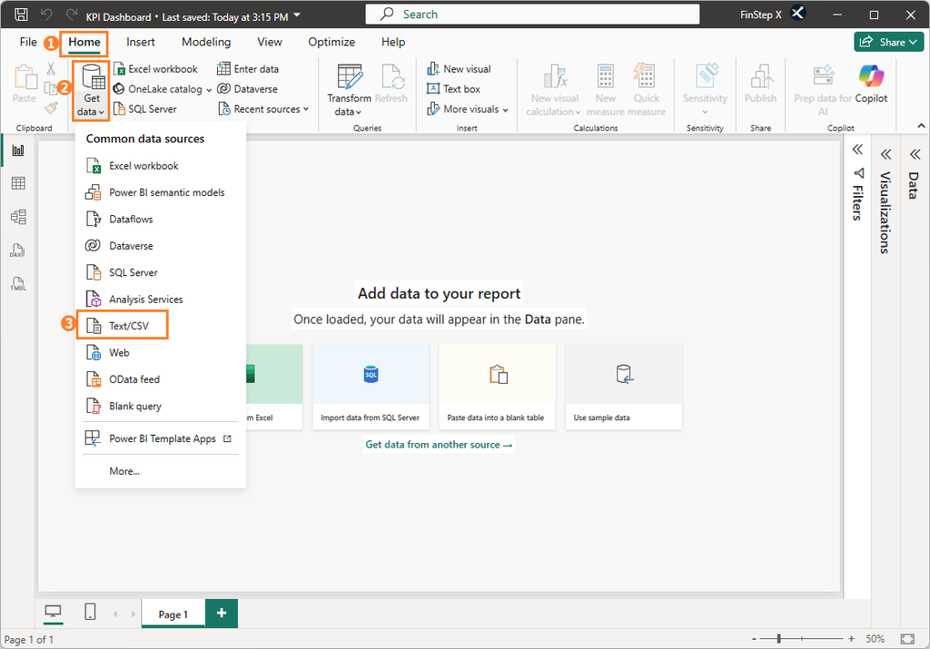
Go to Home → Get data → Text/CSV.
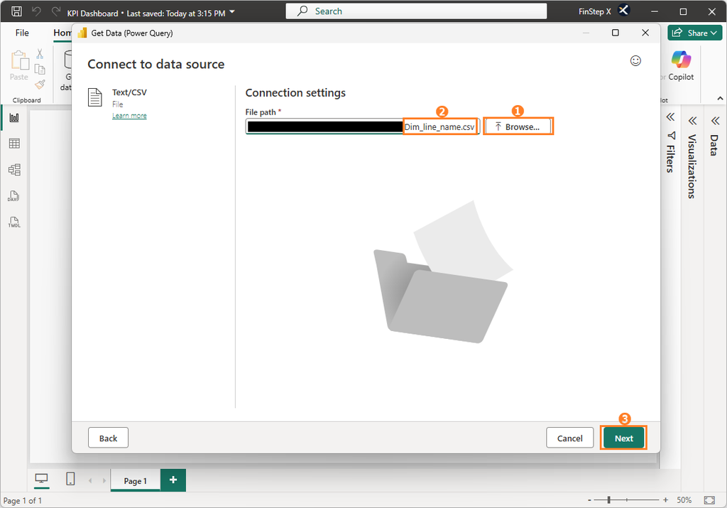
In the Connect to data source window, click Browse, select the first sample file of Dim_line_name.csv from the appropriate folder, and click Open. Then click Next.
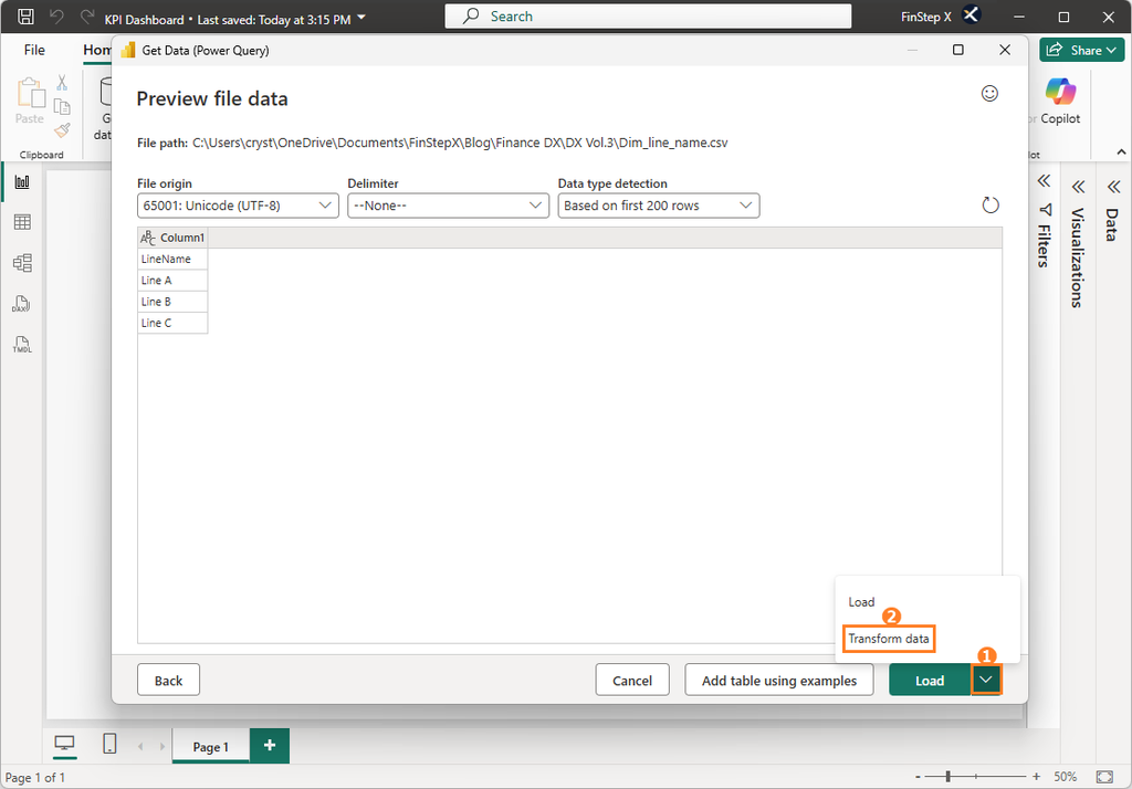
The Preview file data window will appear.
The first row has not been recognized as the column headers, we will not load the data directly. Instead, click the drop-down arrow next to the Load button and select Transform data.
Step 3: Set the Header and Column Names
The Power Query Editor will open. You will see the Queries pane on the left, the Query Settings pane on the right, and a data Preview in the center.
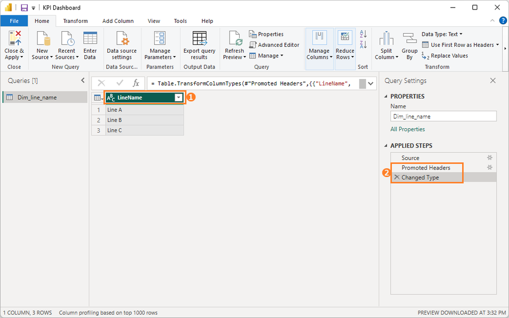
1. Use the First Row as Headers
With the column selected, go to the Home tab and click Use First Row as Headers.
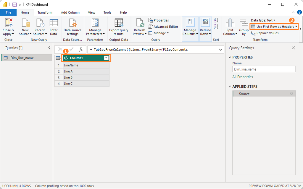
You can now confirm that LineName has been set as the column name. This transformation is recorded in the Applied Steps section on the right side of the screen.
One of the key features of Power Query is that transformation operations are saved as a sequence of steps. When the same data source is refreshed later, these steps can be automatically reapplied in the same order.
2. Rename the Column
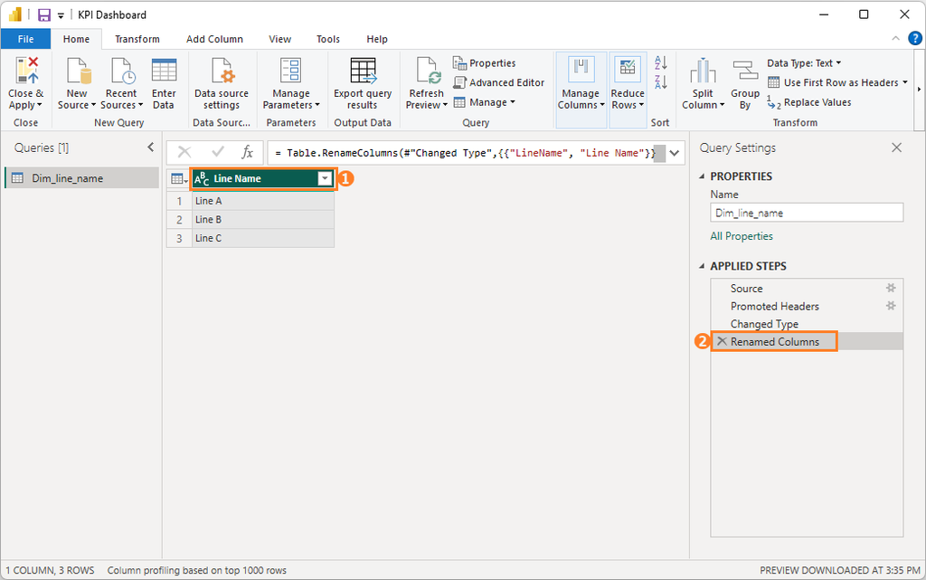
The other sample tables use Line Name as the column name for the production line. To keep the naming consistent, we will rename the column in the production line master table as well.
Double-click the column name LineName, insert a space between the two words, and change it to Line Name. The column rename operation will also be recorded in Applied Steps.
Step 4: Import the Remaining Four CSV Files
Next, let’s add the remaining four CSV files to Power Query.
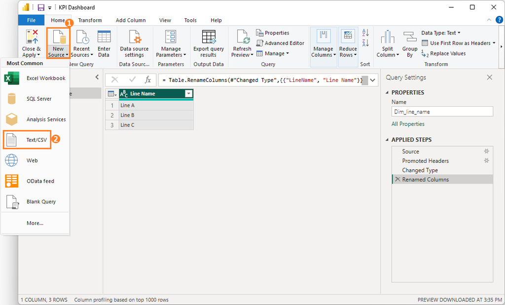
In the Power Query Editor, go to Home → New Source → Text/CSV, and import the following files one at a time:
Fact_monthly_kpi.csvFact_equipment_utilization.csvFact_inventory_turnover.csvFact_defect_rate.csv
For each imported file, check that the column names are correct. If necessary, use the same process described in Step 3 to set the headers and rename columns.
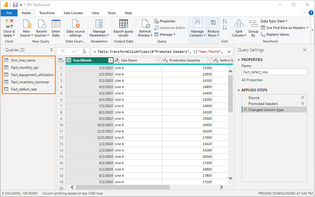
Once all five files have been imported, you will see five queries in the Queries pane.
Step 5: Check the Imported Data
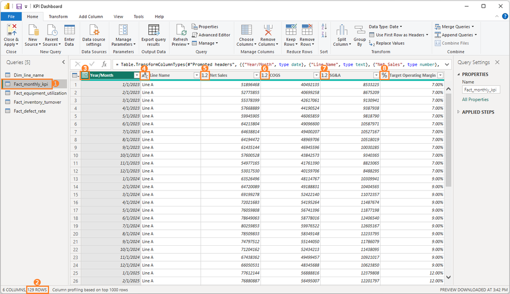
Once the data has been imported, check the number of rows and the data types.
We will use the Fact_monthly_kpi table as an example.
1. Check the Number of Rows
Checking the row count is an important step to make sure that no data is missing.
In the Queries pane of Power Query Editor, select the Fact_monthly_kpi table. Check the row count displayed in the lower-left corner of the screen. For this sample dataset, the correct number is 129 rows. If the row count is different from what you expect, check the applied steps for filters, deleted rows, or other transformations that may have affected the data.
2. Check the Data Types
Incorrect data types can cause unexpected results in later DAX calculations and relationship settings, so it is important to verify them before proceeding.
The following are some of the main data types used in Power BI:
- Calendar icon: Date
- ABC: Text
- 123: Whole Number
- 1.2: Decimal Number
- %: Percentage
Check the data type icon displayed to the left of each column to make sure the correct data type has been assigned. If a data type is incorrect, click the data type icon and select the appropriate data type.
Step 6: Close and Apply
Once you have finished importing the CSV files, setting the headers and column names, and checking the row counts and data types, click Close & Apply on the Home tab.
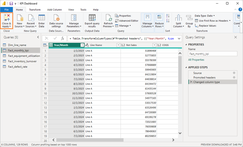
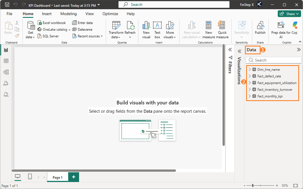
The Power Query Editor will close, and the five tables will appear in the Data pane of Power BI Desktop.
The data import is now complete, and the transformations you made in Power Query have been applied to the Power BI data model.
Step 7: Save the File
Once you have completed the steps above, press Ctrl + S to save the Power BI file.
From the next article onward, we will continue building the report using this KPI Dashboard.pbix file.
Summary
In this article, we imported five CSV files into Power Query and prepared the data by modifying the headers, column names, and checking row counts, and data types.
The main steps we conducted were:
- Save the Power BI file
- Import the CSV files
- Set and rename headers and column names
- Check row counts and data types
- Apply the changes to Power BI
In the next article, we will use the tables imported here to create a Calendar table and configure relationships between the tables.
Frequently Asked Questions (FAQ)
1. What does “Dim” mean in a master table name?
Dim is short for Dimension and is commonly used to identify tables containing descriptive or attribute data, such as master data.
Fact is commonly used for tables containing measurable business data, such as revenue, costs, and utilization rates.
These naming conventions are not mandatory, but they are widely used because they make the role of each table easier to understand.
2. Why should I choose “Transform data” instead of “Load” when importing a CSV file into Power BI?
Load imports the data directly into Power BI.
Transform data opens the data in Power Query, allowing you to clean and transform it before loading it into Power BI.
For real-world data preparation, Transform data is generally the more useful option because you can review and prepare the data before it enters the data model.
3. Can I import multiple CSV files into Power BI at once?
If the files have the same structure, you can use the Folder connector to load all files from a folder.
The five CSV files in this series have different structures, so we import them individually.
4. Why are data types important in Power BI?
Data types affect how data is calculated and how relationships between tables are configured.
For example, Date data types are important for time-based analysis, while numeric data types are required for many DAX calculations.
5. Why do we set the “Year/Month” column to the Date data type?
We set Year/Month to the Date data type so that it can later be used to establish a relationship with the Calendar table.
What’s Next?
In Vol. 4, we will create a Calendar table, establish relationships between the tables, and build the data model for our Power BI report.